Our compiler for PxdScript differs a bit from the examples given above in that it
doesn't compile to machine code which can run directly on the computers hardware.
Instead it compiles to the instruction set of a virtual machine which
is then emulated by the hardware/OS specific platform on which the virtual
machine runs. In other words, the virtual machine is a program written
specifically for a certain platform - in our case for Windows - which can read in
a compiled file containing a PxdScript program and execute the program.
This is not as unusual as you might think - JAVA for example is a language designed
to run on virtual machines (the JVM). You might have heard that JAVA is a platform
independent language and that every JAVA program can run on a wide range of computer
systems. This is also true - the .class files that the JAVA compiler emits contains byte
code which can run on many different systems like Windows, Linux, Mac etc.
But remember that the .class files does not execute directly on the
platforms. You cannot simply type in the name of a .class file in a DOS prompt and
have it execute under Windows. Instead you have to run the .class file by using another
programs - the JVM or "Java Virtual Machine" - by typing 'java myprog.class' at the
prompt.
The file 'java.exe' is a program compiled specifically for Windows and it cannot be
run on other platforms. The reason why the 'myprog.class' program can run on many
different platforms is that similar programs to 'java.exe' exist on all these platforms.
The power of a virtual machine is that once it has been implemented on a specific
platform then we can forget that the language is emulated and consider the virtual
machine as valid and 'physical' as the one on which the virtual machine runs. It has
become a layer of higher abstraction through which we can operate the physical hardware.
It is for example not important to the JAVA programmer that the compiled file doesn't
execute directly on the different machines - the only thing important is that the
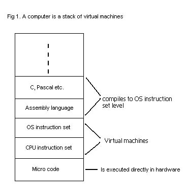
program solves the problem it was designed to solve. As a matter of fact the computer
as we know it is already build up from a stack of virtual machines each emulating
a language of higher level than the one on the level below it. At the very bottom
we have the CPU which provides its users with a certain instruction set. This set
typically contains instructions such as addition, subtraction etc. But even these
seemingly singular instructions (we usually consider the addition of two numbers as
a single operation) is actually 'virtual' instructions emulated by micro programs which
controls the different transistors, registers and gates inside the CPU. The "VM" for
these micro programs is implemented in hardware on the CPU. The different OS runs
on top of these CPU instructions and provides the user with instructions of a higher
level such as instructions to handle files without having to manually specify which
physical disk-blocks on the hard disk that you wish to access. It is more convenient
to be able to type 'fopen("myfile.txt", "tr");' instead of having to tell the hard
disk to start its motors, tell it which disk block we want to access etc. - and we
are able to do that because the OS provides us with an emulated instruction 'fopen'.
On top of the OS we have the assembly language which provides the user
with a programming interface which is easier to read than pure machine code (i.e..
hex numbers in a file) and on top of that we have the high-level languages we know
such as C, Pascal etc. to further simplify the task of programming.
These last 2 layers are different in that they are not emulated by the layer below
them - instead they are compiled into machine code using the OS instruction
set - that is, they are converted from a high-level language to the
low-level language defined by the OS instruction set.
Each new layer in the stack is added to make the computer easier to work with. It
is for example much easier to write code in C than in assembly (in most peoples opinion
at least). If one wish to do so, one is free to add a new layer on top of the stack
- and this is what we're going to do with PxdScript. PxdScript is going to be emulated
by a VM written in C/C++ - a language one level below PxdScript in the stack.
There is still another difference between languages like C or Pascal and PxdScript. Languages like C is (as mentioned above) compiled into machine code on OS level and as far as we are concerned they execute directly on our computer. Languages like PxdScript and JAVA are compiled to something called byte codes which can not be executed directly but instead the meaning of the code must be interpreted by an interpreter as the program execute. A program compiled to machine code is loaded into memory and then the CPU begins to execute the program instruction by instruction. Interpreted code can also be placed totally in memory but it must be 'fed' to the CPU one instruction at a time by the interpreter. The overall operation of an interpreter is very simple and looks like the following loop:
Get next byte code instruction from memory or disk.
Process the byte code and convert to OS instruction level, possibly reading in arguments.
Execute the converted instruction on the CPU using one or more instructions on OS level.
If more byte codes remains, repeat from 1.
And this is in a nutshell how we will code our virtual machine to execute PxdScript programs in chapter 11 when we have the final compiled byte code - only we will not convert the PxdScript instructions to OS level code but simply match them with corresponding functions within our game engine (which of course in the end is converted to OS level code by the C/C++ compiler we use for our game engine).
So far I have just said that PxdScript will run on a VM and that it will compile to
an instruction set defined by that VM - but I haven't described how the instruction
set is defined or how the virtual machine runs the programs. The VM will be a
so-called stack-based machine which is different from for example a
PC which is register-based. The difference is perhaps best described
through an example - the addition of two numbers.
Those of you who has written some assembly code before knows that to add two numbers
on a PC we would first place the numbers in two registers and then add those. Something
like this:
mov ax, 5 ; move 5 into the ax register
mov bx, 8 ; move 8 into the bx register
add ax, bx ; add the content of bx to ax<
Notice that to add the numbers we would have to find two unused registers to hold
our values. The PC only has a very limited number of registers available for general
purposes (ax,bx,cx and dx) so one has to be very careful about how one uses the registers.
It is for example not possible to hold 100 different numbers in the registers at the
same time. If there are no more free registers then we will have to save the value
of some registers to memory and read them back later. This limitation is due to the
fact that the registers we use for the operation represents actual physical registers
inside the CPU - and the number of those are of course limited.
Because PxdScript runs on a virtual machine we do not have to suffer from such limitations.
Our VM is an imaginary machine and if we wanted to do so we could define it to have
thousands of registers (we could easily emulate them by using the disk and some addressing
scheme - right?). But as it turns out using registers is not necessarily the best
way to do it. It is for example quite complicated for the compiler to figure out which
registers to use - even if we had virtually infinitely many. Instead we define the
VM to run using a stack for all its calculations. Again let me demonstrate through
an example:
ldc_int 5 ; load constant '5' and put on stack. Stack is now : 5
ldc_int 8 ; load constant '8' and put on stack. Stack is now : 5,8
iadd ; pop two int's from stack, add them and
push the result. Stack is now : 13
The little snippet of assembly above is actually how the PxdScript compiler generates code for the simple expression '5 + 8'. Notice how the meaning of the assembly code is perfectly clear - without the use of any registers! I'll show you the code for a larger expression so you can get a little more used to the concept of stack-based calculations '(5 + 8)*5 - 4'.
ldc_int 5 ; Stack : 5
ldc_int 8 ; Stack : 5,8
iadd ; Stack : 13
ldc_int 5 ; Stack : 13,5
imul ; Stack : 65
ldc_int 4 ; Stack : 65,4
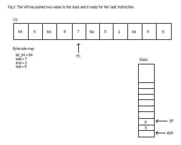
isub ; Stack : 61
So the VM does all its calculations on a stack. But how does it store its variables then? Well, also on the stack actually! The number of variables is something we can calculate at compile time and then reserve space for them at the bottom of the stack. This is one of the things we will calculate in the code for today's chapter! So the variables are numbered from 1 and up, starting with the formals (the parameters to a function - remember?) and then the variables in the body of the code as we reach them. So if for example we calculate that we have 7 different variables then we reserve 7 stack-spaces for variables and start our calculations at stack position 8. We can then load a variable to the top of the stack with the 'iload' instruction and save the top-most stack item to a variable with the 'istore' instruction. Examples:
iload 3 ; Load the 3rd variable to the top of the stack
istore 3 ; save the top-most stack item to variable number 3
Ok, so that is how calculations are done and how variables are stored - but what about
the byte code itself? The above examples has been byte code in symbolic form.
Each of the instructions above like 'ldc_int', 'iadd' etc. has a corresponding number.
As the name implies this number is a byte so the VM can only have 256 different instructions
in its instruction set. As you shall see this is more than enough so there is no need
to worry!! The assembling from byte code in symbolic form to byte code in binary form
is fairly simple - we simply convert the symbolic tokens to their byte number and
save that to a binary file. The arguments to the instructions are saved in a similar
way (but more on this in the next chapter on code generation).
Eventually the code is represented as a stream of bytes. In our VM I will call the
space where the actual byte code lies 'CS' (code segment). The VM has a pointer into
this space called 'PC' (Program Counter) which points out the next instruction to
be interpreted. The program progresses like described in the section on interpreters
- it reads the byte pointed at by the PC, possibly reads arguments to that byte code
instruction and advances the PC accordingly. Then based on the byte code instruction
read it might update the stack.
The stack also have a few pointers associated with it - namely the 'SP' (Stack Pointer)
which always points to the top of the stack and the 'BSP' (Base Stack Pointer) which
points to the base of the stack. The BSP is used in function calling and to access
variables. Remember that I said the bottom positions of the stack was used for variables,
so to get variable 2 we simply access the stack at 'BSP + 2'.
Look at the drawing below to get a better idea of how the VM would represent the code
snippet for '(5 + 8)*5 - 4'.
Ok, enough about the VM for now but know that we will return to it in MUCH greater detail in the next chapter on code generation. In that chapter you will find a complete list of the byte code instructions used and their effect on the stack but for now the important thing is just that you understand the basics of how the VM operates and understands the difference between byte code in symbolic form and byte code in binary form. In symbolic form it looks like assembly code but in binary form it looks like machine code and is 'unreadable' by humans (not true, but it's not so easily done) - however the difference between the two forms is very minor.
Finally it's possible for me to explain what we are trying to calculate in this chapters
module! First of all we wish to calculate the number of variables used in the different
programs and functions and map each variable to a number which will be its address
in the stack. If you look in the 'tree.h' file and find the FUNCTION structure you
will see that it has a field called 'localslimit'. After this module it must contain
the number of variables used in that function. A similar field is found in the PROGRAM
structure.
Now find the structure DECL (for 'variable declaration') in 'tree.h'. Notice that
for all kind of declarations it contains a field called 'offset'. After this module
this field must contain the offset relative to the BSP where the variable is found.
When these fields are all filled out we have completed our first goal and has calculated
what we need to know to create the correct byte code for variable access in the next
chapter.
The second thing we will calculate today is a mapping from labels to
addresses. I haven't mentioned labels yet but obviously some sort of labeling scheme
combined with certain jump instructions is needed to create linear assembly code for
things like conditional statements (for example it is needed to program the 'if-then-else'
construct). Let's look at an example. What follows is the byte code (in symbolic form)
for the 'is equal' construct - that is, expressions such as (a == b). This is a Boolean
operation and based on whether or not the two operands are equal the VM must place
a 0 (for false) or 1 (for true) on top of the stack:
iload_1
; Load the first argument (variable 1)
iload_2
; Load the second argument (variable 2)
if_icmpeq true ; Pop two stack items and
compare them. If equal jump to label 'true'
iconst_0
; If we get here they were NOT equal. Place 0 (false) on stack.
goto stop
; Unconditional jump to label 'stop'
true:
iconst_1
; If we get here they were equal. Place 1 (true) on stack.
stop:
Look through the assembly above and notice that no-matter how you set the values of
variable 1 and 2 then the result will be that either a 0 or a
1 is placed on the stack and the PC will in both cases end at the label 'stop'.
While the block above is easy to read it is not enough when the code is represented
as binary byte code. In binary mode the arguments to the jump instructions are addresses into
the CS - that is, the address the PC (Program Counter) should be moved to. Thus all
labels must be unique and eventually mapped to an offset into the block of memory
we use as CS. For now it is enough that we translate the labels into numbers unique
to the function or program in which they appear. Later when we link the
different functions and programs into the same CS we will change the labels into absolute
addresses into the CS.
Let's address the two issues one at a time:
It should come as no surprise by now that we do the resource calculation by making
a recursive run through the AST. So we start at the top-most node which is the SCRIPTCOLLECTION
node. Eventually we will reach either a function or a program. The offset calculation
is almost identical in both cases - except for the fact that programs cannot have
any formals (parameters). I'll guide you through the resource calculation for a function
(the resFUNCTION() function).
Notice in the top of the file 'resource.c' I declare a global variable called 'offset'
and another called 'localslimit'. Also notice the function 'nextoffset' which does
nothing more than increase the offset variable and return it. It also makes sure the
'localslimit' variable at all times is set to the greatest offset so far. The first
thing we do when we reach a FUNCTION node is to reset the global variables to 0. This
is because the offsets we want is local to the current function or program (each program
and function will operate on its own stack as you will see in a later chapter).
Now we recurse on any formals the function might have. This is the first time we might
reach the function 'resDECL()' which is the most important function for calculating
offsets.
void resDECL(DECL *d) {
switch(d->kind){
case formalK:
d->val.formalD.offset = nextoffset();
break;
case variableK:
/* at this point no difference because of weeding */
d->val.variableD.offset = nextoffset();
if(d->val.variableD.initialization != NULL)
resEXP(d->val.variableD.initialization);
break;
case simplevarK:
d->val.simplevarD.offset = nextoffset();
if(d->val.simplevarD.initialization != NULL)
resEXP(d->val.simplevarD.initialization);
break;
}
if(d->next != NULL)
resDECL(d->next);
}
Important or not - as you can see it is a very very simple function. I think now is
a good time to re-discuss the difference between the 3 variable types 'formalK', 'variableK',
'simplevarK'.
The variables of type 'formalK' are formals (or arguments if you prefer)
to a function and they are special in that each declaration of a formal can only have one identifier
(a formal declaration cannot be 'int a,b,c' and they cannot have any initialization
(we do not support default values for parameters to functions). Formals are the simplest
possible variable declaration.
The variables of type 'variableK' are the normal kind of variable declarations
you find in the body of a function or program. They can be a list of declarations,
have initializations etc. An example could be 'int a,b,c = 0' which is a single declaration
of type 'variableK' which declares 3 different variables and initializes all of them
to 0.
The variables of type 'simplevarK' are variable declarations which can
have initializations - but there can only be one identifier. I.e.. you
cannot declare more than one variable at a time using 'simplevarK' declarations. The
'simplevarK' declaration is used in the FORINIT node - that is the initialization
to a for-loop. Here ',' is used to separate the different parts of the initialization
so it wouldn't make sense to allow declarations of type 'variableK'. So 'simplevarK'
is used for things like: 'for (int a=0, a < 8, a = a+1)'.
As you can see the two cases 'variableK' and 'simplevarK' are treated exactly the
same in the code above. So it would seem that we would miss any additional variables
besides the first one in a 'variableK' declaration because we do not recurse on the
'next' pointer in the IDENTIFIER node. But remember the weeding phase - in that phase
we converted every declarations of type 'variableK' which had more than one identifier
into a list of 'variableK' declarations of only one identifier. I.e.. we converted 'int
a,b,c=0' into 'int a=0; int b=0; int c=0'.
Ok, but in any case what the function does is to pull the next offset number from
the offset-automaton and assign that number to the variable :)
Not much else is happening in the code for offset calculation - follow the recursion
in the AST yourself.
There is only one more subtle point to the calculation: Look at the 'scopeK' case
in the function 'resSTM()':
case scopeK:
/* Notice how we save offset to be able to go back to it */
baseoffset = offset;
resSTM(s->val.scopeS.stm);
offset = baseoffset;
break;
We save the offset value before we enter the scope and set the value back after we leave? Why do we do this? Actually this is not strictly necessary - but it is an optimization which saves us some space on the stack. Remember that we can only see variables in our own scope and scopes higher than our level. Thus, when the PC leaves a scope all variables declared inside that scope cannot ever be reached again and we might as well override their values by reusing their address in the stack. Look at this example to get the idea:
int var1 = 1; // offset 1
int var2 = 2; // offset 2
while (var1 < 8) {
int var3 = 3; // offset 3
int var4 = 4; // offset 4
var1 = var1 + 1;
}
int var5 = 5; // offset 3
When we reach the declaration of 'var5' we are through using variables 'var3' and 'var4' and we might as well reuse their addresses for new variables. If we had not saved the value before entering the scope of the while-loop and set it back afterwards the variable 'var5' would have gotten the offset 5 even though we would never again use the addresses 3 and 4.
Calculating label addresses is even easier than calculating the variable offsets because here there are NO special cases. Like with the offsets we have a function to get the next label and like with offsets we reset the label count every time we reach a function or program. Then we recurse through the body of the function or program and insert label values where needed.
case equalsK:
e->val.equalsE.truelabel = nextlabel();
e->val.equalsE.stoplabel = nextlabel();
resEXP(e->val.equalsE.left);
resEXP(e->val.equalsE.right);
break;
We simply pull two label addresses from the label-automaton and recurse on the expressions (which might contain labels of their own). Every other place where labels are needed works the same way. Look through the code to get the idea.
We finally started working on the back-end of our compiler. This particular chapter
had a lot of easy code but never the less it was quite a challenge for me to write
because there were so many places where I felt I needed to explain stuff which belongs
more to the next two chapters. For example, I touched the subject of code generation
a little in my description of the VM which also had to include some stuff I had planned
to push off until chapter 11 on the VM. The problem is that the 3 topics are so closely
related that I found myself wondering how I learned this stuff myself - it seems that
to understand one part you also have to understand the other two ;)
I hope the result is not too messy and that you can find head and tail in my explanation.
If there is something you find very unclear I would like to hear about it because
it is possible I skipped the explanation of something which seems obvious to me -
but makes part of this text look like it was written in alien for you guys. Stay tuned
for the next chapter which should be out soon (and which will be quite short because
we covered part of it here already).
Keep on codin'
Kasper Fauerby
www.peroxide.dk